
Polars
<div id="qe-notebook-header" align="right" style="text-align:right;"> <a href="https://quantecon.org/" title="quantecon.org"> <img style="width:250px;display:inline;" width="250px" src="https://assets.quantecon.org/img/qe-menubar-logo.svg" alt="QuantEcon"> </a> </div>
19Polars
In addition to what’s in Anaconda, this lecture will need the following libraries:
!pip install --upgrade polars yfinanceOutput
Collecting polars
  Downloading polars-1.43.1-py3-none-any.whl.metadata (11 kB)
Collecting yfinance
  Downloading yfinance-1.5.2-py2.py3-none-any.whl.metadata (6.2 kB)
Collecting polars-runtime-32==1.43.1 (from polars)
  Downloading polars_runtime_32-1.43.1-cp310-abi3-manylinux_2_17_x86_64.manylinux2014_x86_64.whl.metadata (1.5 kB)
Requirement already satisfied: pandas>=1.3.0 in /opt/hostedtoolcache/Python/3.12.13/x64/lib/python3.12/site-packages (from yfinance) (3.0.5)
Requirement already satisfied: numpy>=1.16.5 in /opt/hostedtoolcache/Python/3.12.13/x64/lib/python3.12/site-packages (from yfinance) (2.4.6)
Requirement already satisfied: requests>=2.31 in /opt/hostedtoolcache/Python/3.12.13/x64/lib/python3.12/site-packages (from yfinance) (2.34.2)
Collecting multitasking>=0.0.7 (from yfinance)
  Downloading multitasking-0.0.13-py3-none-any.whl.metadata (16 kB)
Requirement already satisfied: platformdirs>=2.0.0 in /opt/hostedtoolcache/Python/3.12.13/x64/lib/python3.12/site-packages (from yfinance) (4.11.0)
Collecting pytz>=2022.5 (from yfinance)
  Downloading pytz-2026.3.post1-py2.py3-none-any.whl.metadata (22 kB)
Collecting peewee>=3.16.2 (from yfinance)
  Downloading peewee-4.2.6-py3-none-any.whl.metadata (10 kB)
Requirement already satisfied: beautifulsoup4>=4.11.1 in /opt/hostedtoolcache/Python/3.12.13/x64/lib/python3.12/site-packages (from yfinance) (4.15.0)
Collecting curl_cffi>=0.15 (from yfinance)
Downloading curl_cffi-0.15.0-cp310-abi3-manylinux2014_x86_64.manylinux_2_17_x86_64.whl.metadata (18 kB)
Collecting protobuf>=3.19.0 (from yfinance)
  Downloading protobuf-7.35.1-cp310-abi3-manylinux2014_x86_64.whl.metadata (595 bytes)
Collecting websockets>=13.0 (from yfinance)
  Downloading websockets-17.0-cp312-cp312-manylinux1_x86_64.manylinux_2_28_x86_64.manylinux_2_5_x86_64.whl.metadata (6.3 kB)
Requirement already satisfied: soupsieve>=1.6.1 in /opt/hostedtoolcache/Python/3.12.13/x64/lib/python3.12/site-packages (from beautifulsoup4>=4.11.1->yfinance) (2.9.1)
Requirement already satisfied: typing-extensions>=4.0.0 in /opt/hostedtoolcache/Python/3.12.13/x64/lib/python3.12/site-packages (from beautifulsoup4>=4.11.1->yfinance) (4.16.0)
Requirement already satisfied: cffi>=2.0.0 in /opt/hostedtoolcache/Python/3.12.13/x64/lib/python3.12/site-packages (from curl_cffi>=0.15->yfinance) (2.1.0)
Requirement already satisfied: certifi>=2024.2.2 in /opt/hostedtoolcache/Python/3.12.13/x64/lib/python3.12/site-packages (from curl_cffi>=0.15->yfinance) (2026.7.22)
Collecting rich (from curl_cffi>=0.15->yfinance)
  Downloading rich-15.0.0-py3-none-any.whl.metadata (18 kB)
Requirement already satisfied: pycparser in /opt/hostedtoolcache/Python/3.12.13/x64/lib/python3.12/site-packages (from cffi>=2.0.0->curl_cffi>=0.15->yfinance) (3.0)
Requirement already satisfied: python-dateutil>=2.8.2 in /opt/hostedtoolcache/Python/3.12.13/x64/lib/python3.12/site-packages (from pandas>=1.3.0->yfinance) (2.9.0.post0)
Requirement already satisfied: six>=1.5 in /opt/hostedtoolcache/Python/3.12.13/x64/lib/python3.12/site-packages (from python-dateutil>=2.8.2->pandas>=1.3.0->yfinance) (1.17.0)
Requirement already satisfied: charset_normalizer<4,>=2 in /opt/hostedtoolcache/Python/3.12.13/x64/lib/python3.12/site-packages (from requests>=2.31->yfinance) (3.4.9)
Requirement already satisfied: idna<4,>=2.5 in /opt/hostedtoolcache/Python/3.12.13/x64/lib/python3.12/site-packages (from requests>=2.31->yfinance) (3.18)
Requirement already satisfied: urllib3<3,>=1.26 in /opt/hostedtoolcache/Python/3.12.13/x64/lib/python3.12/site-packages (from requests>=2.31->yfinance) (2.7.0)
Collecting markdown-it-py>=2.2.0 (from rich->curl_cffi>=0.15->yfinance)
  Downloading markdown_it_py-4.2.0-py3-none-any.whl.metadata (7.4 kB)
Requirement already satisfied: pygments<3.0.0,>=2.13.0 in /opt/hostedtoolcache/Python/3.12.13/x64/lib/python3.12/site-packages (from rich->curl_cffi>=0.15->yfinance) (2.20.0)
Collecting mdurl~=0.1 (from markdown-it-py>=2.2.0->rich->curl_cffi>=0.15->yfinance)
  Downloading mdurl-0.1.2-py3-none-any.whl.metadata (1.6 kB)
Downloading polars-1.43.1-py3-none-any.whl (846 kB)
   ━━━━━━━━━━━━━━━━━━━━━━━━━━━━━━━━━━━━━━━━ 0.0/846.8 kB ? eta -:--:--
━━━━━━━━━━━━━━━━━━━━━━━━━━━━━━━━━━━━━━━━ 846.8/846.8 kB 38.6 MB/s 0:00:00
Downloading polars_runtime_32-1.43.1-cp310-abi3-manylinux_2_17_x86_64.manylinux2014_x86_64.whl (57.3 MB)
━━━━━━━━━━━━━━━━━━━━━━━━━━━━━━━━━━━━━━━━ 0.0/57.3 MB ? eta -:--:-- ━━━━━━━━━━━━━━━━━━━━━━━━━━━━━━╸━━━━━━━━━ 43.8/57.3 MB 218.6 MB/s eta 0:00:01 ━━━━━━━━━━━━━━━━━━━━━━━━━━━━━━━━━━━━━━━━ 57.3/57.3 MB 151.9 MB/s 0:00:00
Downloading yfinance-1.5.2-py2.py3-none-any.whl (144 kB)
Downloading curl_cffi-0.15.0-cp310-abi3-manylinux2014_x86_64.manylinux_2_17_x86_64.whl (11.1 MB)
━━━━━━━━━━━━━━━━━━━━━━━━━━━━━━━━━━━━━━━━ 0.0/11.1 MB ? eta -:--:-- ━━━━━━━━━━━━━━━━━━━━━━━━━━━━━━━━━━━━━━━━ 11.1/11.1 MB 239.3 MB/s 0:00:00
Downloading multitasking-0.0.13-py3-none-any.whl (16 kB)
Downloading peewee-4.2.6-py3-none-any.whl (173 kB)
Downloading protobuf-7.35.1-cp310-abi3-manylinux2014_x86_64.whl (327 kB)
Downloading pytz-2026.3.post1-py2.py3-none-any.whl (508 kB)
Downloading websockets-17.0-cp312-cp312-manylinux1_x86_64.manylinux_2_28_x86_64.manylinux_2_5_x86_64.whl (220 kB)
Downloading rich-15.0.0-py3-none-any.whl (310 kB)
Downloading markdown_it_py-4.2.0-py3-none-any.whl (91 kB)
Downloading mdurl-0.1.2-py3-none-any.whl (10.0 kB)
Installing collected packages: pytz, peewee, multitasking, websockets, protobuf, polars-runtime-32, mdurl, polars, markdown-it-py, rich, curl_cffi, yfinance
Successfully installed curl_cffi-0.15.0 markdown-it-py-4.2.0 mdurl-0.1.2 multitasking-0.0.13 peewee-4.2.6 polars-1.43.1 polars-runtime-32-1.43.1 protobuf-7.35.1 pytz-2026.3.post1 rich-15.0.0 websockets-17.0 yfinance-1.5.2
19.1Overview
Polars is a fast data manipulation library for Python written in Rust.
It has gained significant popularity as a modern alternative to Pandas due to its performance advantages.
Polars is designed with performance and memory efficiency in mind, leveraging:
Apache Arrow columnar format for fast data access
Lazy evaluation to optimize query execution
Parallel processing to utilize all available CPU cores
An expressive API built around column expressions
Throughout the lecture, we will assume that the following imports have taken place
import polars as pl
import numpy as np
import matplotlib.pyplot as plt
Like Pandas, Polars defines two important data types: Series and DataFrame.
You can think of a Series as a column of data, such as a collection of observations on a single variable.
A DataFrame is a two-dimensional object for storing related columns of data.
19.2Series
Let’s start with Series.
We begin by creating a series of four random observations
s = pl.Series(name='daily returns', values=np.random.randn(4))
sPolars Series are built on top of Apache Arrow arrays and support many familiar operations
s * 100Absolute values are available as a method
s.abs()We can also get quick summary statistics
s.describe()Since Polars has no row index, labelled data requires a DataFrame.
For example, to associate ticker symbols with returns:
df = pl.DataFrame({
    'company': ['AMZN', 'AAPL', 'MSFT', 'GOOG'],
    'daily returns': np.random.randn(4)
})
dfWe access a value by filtering on a column expression
df.filter(
    pl.col('company') == 'AMZN'
).select('daily returns').item()-1.2198649509859698Updates also use expressions rather than index assignment
df = df.with_columns(
    pl.when(pl.col('company') == 'AMZN')
    .then(0)
    .otherwise(pl.col('daily returns'))
    .alias('daily returns')
)
dfWe can also check membership
'AAPL' in df['company']True19.3DataFrames
While a Series is a single column of data, a DataFrame is several columns, one for each variable.
As in Pandas, let’s work with data from the Penn World Tables.
We read this in using pl.read_csv
url = ('https://raw.githubusercontent.com/QuantEcon/'
       'lecture-python-programming/main/lectures/_static/'
       'lecture_specific/pandas/data/test_pwt.csv')
df = pl.read_csv(url)
df19.3.1Selecting data
We can select rows by slicing and columns by name
df[2:5]To select specific columns, pass a list of names to select
df.select(['country', 'tcgdp'])These can be combined
df[2:5].select(['country', 'tcgdp'])19.3.2Filtering by conditions
The filter method accepts boolean expressions built from pl.col
df.filter(pl.col('POP') >= 20000)Multiple conditions can be combined with & (and) and | (or)
df.filter(
    (pl.col('country').is_in(['Argentina', 'India', 'South Africa'])) &
    (pl.col('POP') > 40000)
)Expressions can involve arithmetic across columns
df.filter(
    (pl.col('cc') + pl.col('cg') >= 80) & (pl.col('POP') <= 20000)
)Select the country with the largest household consumption share
df.filter(pl.col('cc') == pl.col('cc').max())19.3.3Column expressions
A key difference from pandas is that Polars uses column expressions for transformations rather than element-wise apply calls.
Here is an example computing the max of each numeric column
df.select(
    pl.col(['year', 'POP', 'XRAT', 'tcgdp', 'cc', 'cg'])
    .max()
    .name.suffix('_max')
)Expressions can be used inside with_columns to add or modify columns
df.with_columns(
    (pl.col('XRAT') / 10).alias('XRAT_scaled'),
    pl.col(pl.Float64).round(2)
)Conditional logic uses pl.when(...).then(...).otherwise(...)
df.with_columns(
    pl.when(pl.col('POP') >= 20000)
    .then(pl.col('POP'))
    .otherwise(None)
    .alias('POP_filtered')
).select(['country', 'POP', 'POP_filtered'])19.3.4Missing values
Let’s insert some null values to demonstrate imputation techniques
df_nulls = df.with_row_index().with_columns(
    pl.when(pl.col('index') == 0)
    .then(None).otherwise(pl.col('XRAT')).alias('XRAT'),
    pl.when(pl.col('index') == 3)
    .then(None).otherwise(pl.col('cc')).alias('cc'),
    pl.when(pl.col('index') == 5)
    .then(None).otherwise(pl.col('tcgdp')).alias('tcgdp'),
    pl.when(pl.col('index') == 6)
    .then(None).otherwise(pl.col('POP')).alias('POP'),
).drop('index')
df_nullsFill all nulls with zero
df_nulls.fill_null(0)Or fill with column means
cols = ['cc', 'tcgdp', 'POP', 'XRAT']
df_nulls.with_columns(
    pl.col(cols).fill_null(pl.col(cols).mean())
)Polars also supports forward fill (fill_null(strategy='forward')) and interpolation.
There are more advanced imputation tools available in scikit-learn.
19.3.5Visualization
Let’s build a GDP per capita column and plot it
df = (df
    .select(['country', 'POP', 'tcgdp'])
    .rename({'POP': 'population', 'tcgdp': 'total GDP'})
    .with_columns(
        (pl.col('population') * 1e3).alias('population')
    )
    .with_columns(
        (pl.col('total GDP') * 1e6 / pl.col('population'))
        .alias('GDP percap')
    )
    .sort('GDP percap', descending=True)
)
dfWe can extract columns directly for matplotlib
fig, ax = plt.subplots()
ax.bar(df['country'].to_list(), df['GDP percap'].to_list())
ax.set_xlabel('country', fontsize=12)
ax.set_ylabel('GDP per capita', fontsize=12)
plt.xticks(rotation=45, ha='right')
plt.tight_layout()
plt.show()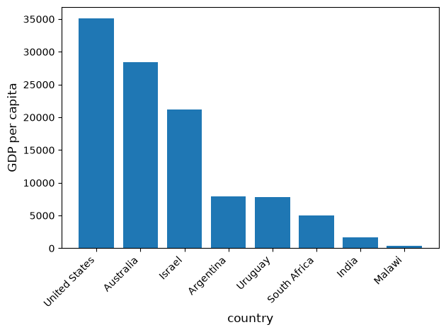
19.4Lazy evaluation
One of Polars’ most powerful features is lazy evaluation.
Instead of executing each operation immediately, lazy mode collects the full query plan and optimizes it before running.
19.4.1Eager vs lazy
# Reload the dataset
url = ('https://raw.githubusercontent.com/QuantEcon/'
       'lecture-python-programming/main/lectures/_static/'
       'lecture_specific/pandas/data/test_pwt.csv')
df_full = pl.read_csv(url)
The eager API executes immediately (like pandas)
result_eager = (df_full
    .filter(pl.col('tcgdp') > 1000)
    .select(['country', 'year', 'tcgdp'])
    .sort('tcgdp', descending=True)
)
result_eager.head()The lazy API builds a query plan instead
lazy_query = (df_full.lazy()
    .filter(pl.col('tcgdp') > 1000)
    .select(['country', 'year', 'tcgdp'])
    .sort('tcgdp', descending=True)
)
print(lazy_query.explain())
SORT BY [descending: [true]] [col("tcgdp")]
FILTER col("tcgdp") > 1000.0
FROM
DF ["country", "country isocode", "year", "POP", ...]; PROJECT["country", "year", "tcgdp"] 3/8 COLUMNS
Call collect to execute the plan
result_lazy = lazy_query.collect()
result_lazy.head()19.4.2Query optimization
The lazy engine applies several optimizations automatically:
Predicate pushdown --- filters are applied as early as possible
Projection pushdown --- only required columns are read from the source
Common subexpression elimination --- duplicate calculations are merged
Let’s see how Polars rewrites a multi-step query
optimized = (df_full.lazy()
    .select(['country', 'year', 'tcgdp', 'POP'])
    .filter(pl.col('tcgdp') > 500)
    .with_columns(
        (pl.col('tcgdp') / pl.col('POP')).alias('gdp_per_capita')
    )
    .filter(pl.col('gdp_per_capita') > 10)
    .select(['country', 'year', 'gdp_per_capita'])
)

print("Optimized plan:")
print(optimized.explain())
Optimized plan:
FILTER col("gdp_per_capita") > 10.0
FROM
simple π 3/3 ["country", "year", ... 1 other column]
WITH_COLUMNS:
[(col("tcgdp") / col("POP")).alias("gdp_per_capita")]
FILTER col("tcgdp") > 500.0
FROM
DF ["country", "country isocode", "year", "POP", ...]; PROJECT["country", "year", "tcgdp", "POP"] 4/8 COLUMNS
Executing the plan gives us the final result
optimized.collect()19.4.3Performance comparison
Let’s compare pandas, Polars eager, and Polars lazy on the same task.
We start with a small dataset (the Penn World Tables we used above) to show that for small data the differences are negligible
import pandas as pd
import time

# Small dataset -- Penn World Tables (~8 rows)
url = ('https://raw.githubusercontent.com/QuantEcon/'
       'lecture-python-programming/main/lectures/_static/'
       'lecture_specific/pandas/data/test_pwt.csv')
small_pd = pd.read_csv(url)
small_pl = pl.read_csv(url)
Now we time the same filter-select-sort operation in each library
# pandas
start = time.perf_counter()
_ = (small_pd
     .query('tcgdp > 500')
     [['country', 'year', 'tcgdp', 'POP']]
     .assign(gdp_pc=lambda d: d['tcgdp'] / d['POP'])
     .sort_values('gdp_pc', ascending=False))
pd_small = time.perf_counter() - start

# Polars eager
start = time.perf_counter()
_ = (small_pl
     .filter(pl.col('tcgdp') > 500)
     .select(['country', 'year', 'tcgdp', 'POP'])
     .with_columns((pl.col('tcgdp') / pl.col('POP')).alias('gdp_pc'))
     .sort('gdp_pc', descending=True))
pl_small = time.perf_counter() - start

print(f"Small data  --  pandas: {pd_small:.4f}s | Polars eager: {pl_small:.4f}s")
Small data -- pandas: 0.0078s | Polars eager: 0.0034s
On a handful of rows the speed difference is immaterial --- use whichever API you find more convenient.
Now let’s scale up to 5 million rows where the difference becomes clear.
The task is: filter rows where value > 0, compute a weighted product
value * weight, then take the mean of that product within each group ---
a grouped weighted average.
n = 5_000_000
np.random.seed(42)

groups = np.random.choice(['A', 'B', 'C', 'D'], n)
values = np.random.randn(n)
weights = np.random.rand(n)
extra1 = np.random.randn(n)
extra2 = np.random.randn(n)

big_pd = pd.DataFrame({
    'group': groups, 'value': values,
    'weight': weights, 'extra1': extra1, 'extra2': extra2
})
big_pl = pl.DataFrame({
    'group': groups, 'value': values,
    'weight': weights, 'extra1': extra1, 'extra2': extra2
})
First, the pandas baseline
start = time.perf_counter()
tmp = big_pd[big_pd['value'] > 0][['group', 'value', 'weight']].copy()
tmp['weighted'] = tmp['value'] * tmp['weight']
_ = tmp.groupby('group')['weighted'].mean()
pd_time = time.perf_counter() - start
print(f"pandas:       {pd_time:.4f}s")
pandas: 0.4301s
Next, Polars in eager mode
start = time.perf_counter()
_ = (big_pl
    .filter(pl.col('value') > 0)
    .select(['group', 'value', 'weight'])
    .with_columns(
        (pl.col('value') * pl.col('weight')).alias('weighted'))
    .group_by('group')
    .agg(pl.col('weighted').mean()))
eager_time = time.perf_counter() - start
print(f"Polars eager: {eager_time:.4f}s")
Polars eager: 0.1002s
And finally, Polars in lazy mode
start = time.perf_counter()
_ = (big_pl.lazy()
    .filter(pl.col('value') > 0)
    .select(['group', 'value', 'weight'])
    .with_columns(
        (pl.col('value') * pl.col('weight')).alias('weighted'))
    .group_by('group')
    .agg(pl.col('weighted').mean())
    .collect())
lazy_time = time.perf_counter() - start
print(f"Polars lazy:  {lazy_time:.4f}s")
Polars lazy: 0.0521s
The take-away:
For small data (thousands of rows), pandas and Polars perform similarly --- choose based on API preference and ecosystem fit.
For medium to large data (hundreds of thousands of rows and above), Polars can be significantly faster thanks to its Rust engine, parallel execution, and (in lazy mode) query optimization.
The lazy API is particularly powerful when reading from disk --- scan_csv returns a LazyFrame directly, so filters and projections are pushed down to the file reader.
19.5On-line data sources
As in Pandas, Python makes it straightforward to query online databases.
An important database for economists is FRED --- a vast collection of time series data maintained by the St. Louis Fed.
Polars’ read_csv can fetch data from a URL directly.
We use try_parse_dates=True to parse the date column automatically
fred_url = ('https://fred.stlouisfed.org/graph/fredgraph.csv?'
            'bgcolor=%23e1e9f0&chart_type=line&drp=0&'
            'fo=open%20sans&graph_bgcolor=%23ffffff&'
            'height=450&mode=fred&recession_bars=on&'
            'txtcolor=%23444444&ts=12&tts=12&width=1318&'
            'nt=0&thu=0&trc=0&show_legend=yes&'
            'show_axis_titles=yes&show_tooltip=yes&'
            'id=UNRATE&scale=left&cosd=1948-01-01&'
            'coed=2024-06-01&line_color=%234572a7&'
            'link_values=false&line_style=solid&'
            'mark_type=none&mw=3&lw=2&ost=-99999&'
            'oet=99999&mma=0&fml=a&fq=Monthly&fam=avg&'
            'fgst=lin&fgsnd=2020-02-01&line_index=1&'
            'transformation=lin&vintage_date=2024-07-29&'
            'revision_date=2024-07-29&nd=1948-01-01')
data = pl.read_csv(fred_url, try_parse_dates=True)
Let’s inspect the first few rows
data.head()And get summary statistics
data.describe()Plot the unemployment rate from 2006 to 2012
filtered = data.filter(
    (pl.col('observation_date') >= pl.date(2006, 1, 1)) &
    (pl.col('observation_date') <= pl.date(2012, 12, 31))
)

fig, ax = plt.subplots()
ax.plot(filtered['observation_date'].to_list(),
        filtered['UNRATE'].to_list())
ax.set_title('US Unemployment Rate')
ax.set_xlabel('year', fontsize=12)
ax.set_ylabel('%', fontsize=12)
plt.show()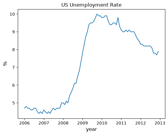
Polars supports many file formats including Excel, JSON, Parquet, and direct database connections.
19.6Exercises
Solution to Exercise 1
Calculate percentage changes using Polars expressions:
price_change = ticker.select([
    ((pl.col(tick).last() / pl.col(tick).first() - 1) * 100)
    .alias(tick)
    for tick in ticker_list.keys()
]).transpose(
    include_header=True,
    header_name='ticker',
    column_names=['pct_change']
).with_columns(
    pl.col('ticker')
    .replace_strict(ticker_list, default=pl.col('ticker'))
    .alias('company')
).sort('pct_change')

print(price_change)
shape: (11, 3)
┌────────┬────────────┬───────────┐
│ ticker ┆ pct_change ┆ company │
│ --- ┆ --- ┆ --- │
│ str ┆ f64 ┆ str │
╞════════╪════════════╪═══════════╡
│ BHP ┆ -2.249076 ┆ BHP │
│ C ┆ 3.550584 ┆ Citigroup │
│ AMZN ┆ 5.845049 ┆ Amazon │
│ INTC ┆ 6.868556 ┆ Intel │
│ KO ┆ 14.922487 ┆ Coca-Cola │
│ … ┆ … ┆ … │
│ TM ┆ 23.416739 ┆ Toyota │
│ QCOM ┆ 25.31854 ┆ Qualcomm │
│ AAPL ┆ 38.550745 ┆ Apple │
│ MSFT ┆ 57.179567 ┆ Microsoft │
│ GOOG ┆ 68.960915 ┆ Google │
└────────┴────────────┴───────────┘
Plot the results using matplotlib directly:
companies = price_change['company'].to_list()
changes = price_change['pct_change'].to_list()
colors = ['red' if x < 0 else 'blue' for x in changes]

fig, ax = plt.subplots(figsize=(10, 8))
ax.bar(companies, changes, color=colors)
ax.set_xlabel('stock', fontsize=12)
ax.set_ylabel('percentage change in price', fontsize=12)
plt.xticks(rotation=45, ha='right')
plt.tight_layout()
plt.show()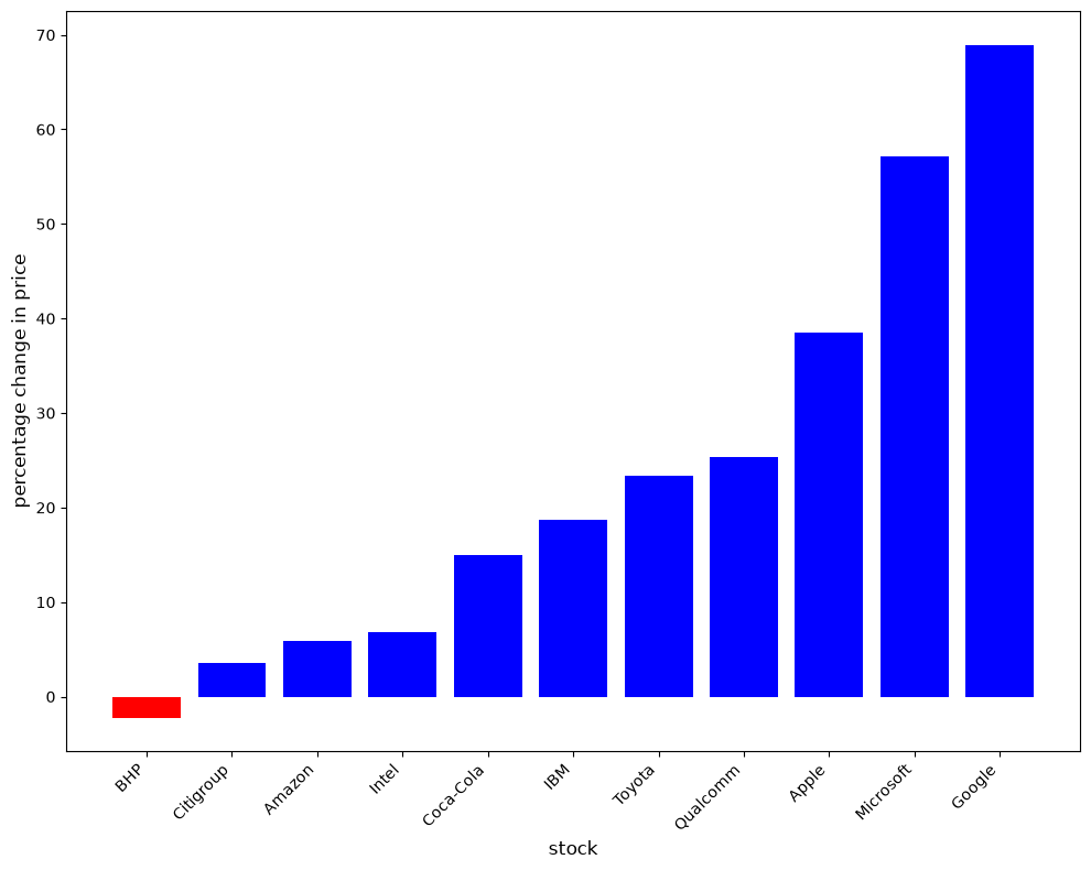
Solution to Exercise 2
indices_data = read_data_polars(
    indices_list,
    start=dt.datetime(1971, 1, 1),
    end=dt.datetime(2021, 12, 31)
)

indices_data = indices_data.with_columns(
    pl.col('Date').dt.year().alias('year')
)
Calculate yearly returns using group-by operations:
yearly_returns = indices_data.group_by('year').agg([
    *[pl.col(idx).drop_nulls().first().alias(f'{idx}_first')
      for idx in indices_list],
    *[pl.col(idx).drop_nulls().last().alias(f'{idx}_last')
      for idx in indices_list]
])

for idx, name in indices_list.items():
    yearly_returns = yearly_returns.with_columns(
        ((pl.col(f'{idx}_last') - pl.col(f'{idx}_first'))
         / pl.col(f'{idx}_first') * 100).alias(name)
    )

yearly_returns = (yearly_returns
    .select(['year', *indices_list.values()])
    .sort('year')
)
print(yearly_returns)
shape: (51, 5)
┌──────┬────────────┬────────────┬───────────┬────────────┐
│ year ┆ S&P 500 ┆ NASDAQ ┆ Dow Jones ┆ Nikkei │
│ --- ┆ --- ┆ --- ┆ --- ┆ --- │
│ i32 ┆ f64 ┆ f64 ┆ f64 ┆ f64 │
╞══════╪════════════╪════════════╪═══════════╪════════════╡
│ 1971 ┆ 12.002188 ┆ 14.120003 ┆ null ┆ 36.407234 │
│ 1972 ┆ 16.110952 ┆ 17.668274 ┆ null ┆ 92.011231 │
│ 1973 ┆ -18.094035 ┆ -31.523435 ┆ null ┆ -17.697016 │
│ 1974 ┆ -29.811633 ┆ -35.350697 ┆ null ┆ -9.914309 │
│ 1975 ┆ 28.4209 ┆ 27.874797 ┆ null ┆ 16.798024 │
│ … ┆ … ┆ … ┆ … ┆ … │
│ 2017 ┆ 18.415027 ┆ 27.155799 ┆ 24.331151 ┆ 16.182267 │
│ 2018 ┆ -7.009394 ┆ -5.303631 ┆ -6.028635 ┆ -14.853703 │
│ 2019 ┆ 28.714796 ┆ 34.603667 ┆ 22.23998 ┆ 20.931737 │
│ 2020 ┆ 15.292907 ┆ 41.751104 ┆ 6.019231 ┆ 18.269064 │
│ 2021 ┆ 29.132182 ┆ 23.964416 ┆ 20.428169 ┆ 5.625169 │
└──────┴────────────┴────────────┴───────────┴────────────┘
Summary statistics:
yearly_returns.select(list(indices_list.values())).describe()Plot each index in a subplot:
fig, axes = plt.subplots(2, 2, figsize=(12, 10))
years = yearly_returns['year'].to_list()

for iter_, ax in enumerate(axes.flatten()):
    name = list(indices_list.values())[iter_]
    values = yearly_returns[name].to_list()
    ax.plot(years, values, 'o-', linewidth=2, markersize=4)
    ax.axhline(y=0, color='k', linestyle='--', alpha=0.3)
    ax.set_ylabel('yearly return (%)', fontsize=12)
    ax.set_xlabel('year', fontsize=12)
    ax.set_title(name, fontsize=12)

plt.tight_layout()
plt.show()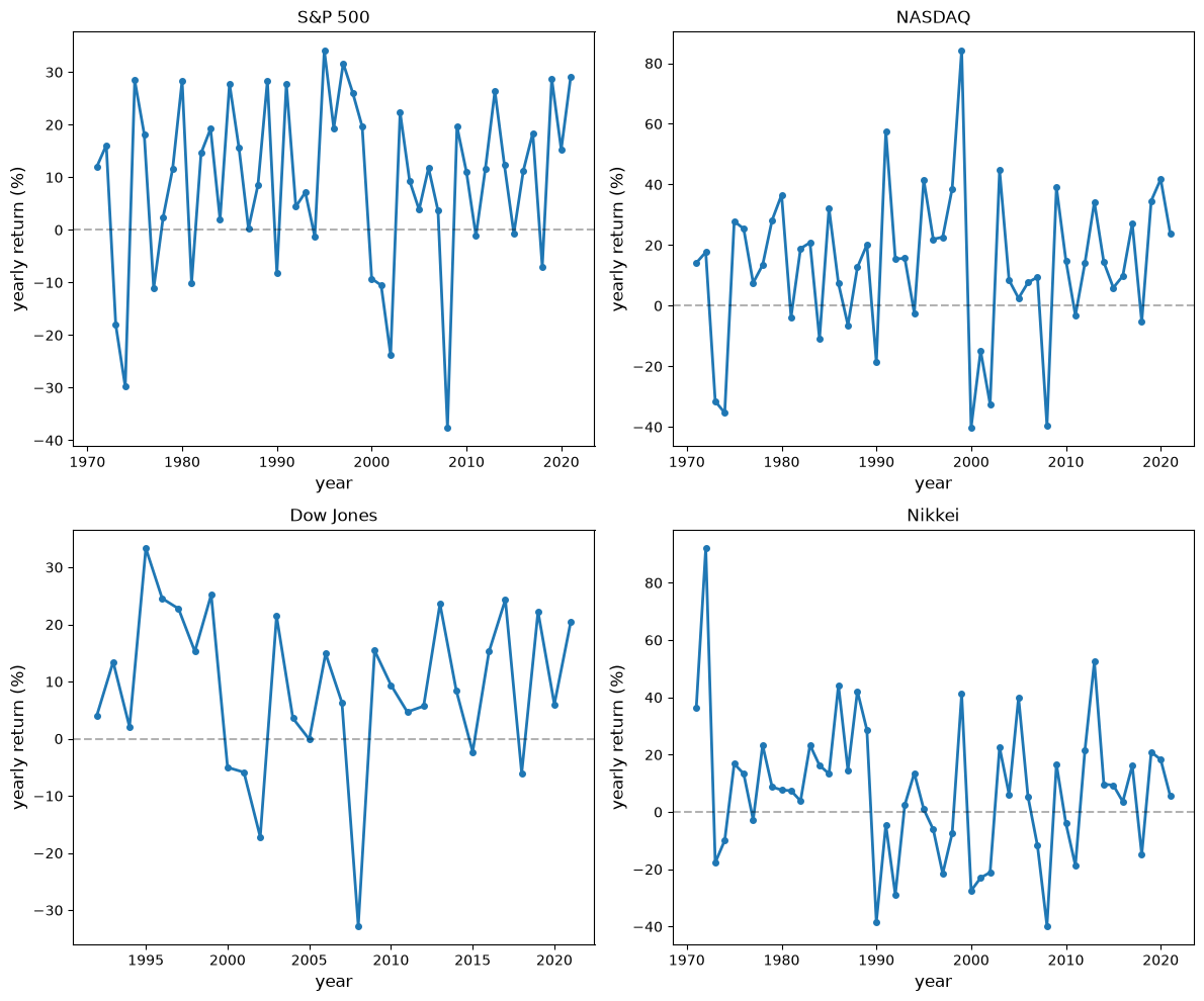

Creative Commons License – This work is licensed under a Creative Commons Attribution-ShareAlike 4.0 International.